$$ \DeclareMathOperator*{\argmin}{\arg\!\min} \DeclareMathOperator*{\argmax}{\arg\!\max} \newcommand\independenT{\protect\mathpalette{\protect\independenT}{\perp}} \def\independenT#1{\mathrel{\rlap{#1}\mkern2mu{#1}}} \newcommand{\rv}[2]{ #1_{1},...,#1_{#2} } \newcommand{\conv}[1]{ \overset{#1}{\longrightarrow} } \newcommand{\dnconv}[1]{ \overset{#1}{\centernot\longrightarrow} } \newcommand\smtop{\mkern-2mu\raise.25ex\hbox{$\scriptscriptstyle\top$}\mkern-3mu} \def\ds{\displaystyle} \def\bs{\boldsymbol} \def\bsl{\backslash} \def\ipl{\langle} \def\ipr{\rangle} \def\st{\text{\indent s.t \indent }} \def\bif{\text{\indent if \indent } } \def\a{\alpha} \def\b{\beta} \def\g{\gamma} \def\th{\theta} \def\bth{\boldsymbol \theta} \def\la{\lambda} \def\La{\Lambda} \def\k{\kappa} \def\t{\tau} \def\r{\rho} \def\s{\sigma} \def\ssq{\sigma^2} \def\d{\delta} \def\w{\omega} \def\om{\Omega} \def\vep{\varepsilon} \def\vphi{\varphi} \def\cL{\mathcal{L}} \def\indi{\mathbbm{1}} \def\I{\mathcal{I}} \def\J{\mathcal{J}} \def\es{\emptyset} \def\var{\mathrm{var}} \def\Var{\mathrm{var}} \def\cov{\mathrm{cov}} \def\sd{\mathrm{sd}} \def\y{\textbf{\textit{y}}} \def\R{\mathbb{R}} \def\Q{\mathbb{Q}} \def\Qc{\mathbb{Q}^{c}} \def\bE{\mathbb{E}} \def\bP{\mathbb{P}} \def\Z{\mathbb{Z}} \def\C{\mathbb{C}} \def\N{\mathbb{N}} \def\H{\mathbb{H}} \def\Sbb{\mathbb{S}} \def\sA{\mathscr{A}} \def\cA{\mathcal{A}} \def\sD{\mathscr{D}} \def\cD{\mathcal{D}} \def\cG{\mathcal{G}} \def\G{\mathscr{G}} \def\F{\mathscr{F}} \def\sR{\mathscr{R}} \def\cB{\mathcal{B}} \def\sB{\mathscr{B}} \def\sC{\mathscr{C}} \def\cC{\mathcal{C}} \def\cE{\mathcal{E}} \def\sE{\mathscr{E}} \def\fF{\mathfrak{F}} \def\sF{\mathscr{F}} \def\fG{\mathfrak{G}} \def\bG{\mathbbm{G}} \def\sG{\mathscr{G}} \def\sH{\mathscr{H}} \def\cH{\mathcal{H}} \def\sJ{\mathscr{J}} \def\cJ{\mathcal{J}} \def\I{\mathcal{I}} \def\J{\mathcal{J}} \def\sT{\mathscr{T}} \def\cT{\mathcal{T}} \def\fM{\mathfrak{M}} \def\cM{\mathcal{M}} \def\sM{\mathscr{M}} \def\cN{\mathcal{N}} \def\sN{\mathscr{N}} \def\sP{\mathscr{P}} \def\cP{\mathcal{P}} \def\cW{\mathcal{W}} \def\X{\mathcal{X}} \def\Y{\mathcal{Y}} \def\cP{\mathcal{P}} \def\sP{\mathscr{P}} \def\SS{\mathscr{S}} \def\ker{\mathrm{ker}} \def\ran{\mathrm{ran}} \def\vecv{\mathrm{vec}} \def\wec{\mathrm{wec}} \def\diag{\mathrm{diag}} \def\sspan{\mathrm{span}} % I think this clashes with something; will not work \def\tr{\mathrm{tr}} \def\rank{\mathrm{rank}} \def\pr{\mathrm{pr}} \def\dist{\mathrm{dist}} \def\BIC{\mathrm{BIC}} \def\KC{\mathrm{KC}} \def\inprob{\overset{p}{\longrightarrow}} \def\indist{\overset{d}{\longrightarrow}} \def\eqdist{\overset{d}{=}} \def\as{\overset{a.s}{\longrightarrow}} \def\tends{\longrightarrow} \def\ind{\;\;\;\;\;} \def\etal{\text{et al.} } \def\indep{\independenT{\perp}} \def\iid{\overset{iid}{\sim}} \def\GEP{\mathrm{GEP}} \def\sspan{\mathrm{span}} \def\bnorm{ \bigg \| } $$

Outer Product of Canonical Gradients

Author

Harris Quach

Published

January 1, 2025

Introduction

Place Holder for OPCG

Sufficient Dimension Reduction (SDR) is an area of statistics that focuses on reducing high dimensional data to a just a few features that reflect, or summarize, all the available information about a specific outcome of interest. In data science parlance, SDR can be considered methods for “supervised dimension reduction” or “supervised learning”.

Ideally, the supervised features will be more interpretable than trying to use the entire set of predictors. Then any subsequent model built upon the supervised features should be more interpretable as well. In terms of interpretability, the supervised features are easier to visualize, since they are lower dimensional summaries and we only have a few to consider. We can plot the supervised features against the outcome in 1d, 2d, and 3d graphics, which can help build a better understanding of the relationship between the outcome and predictors.

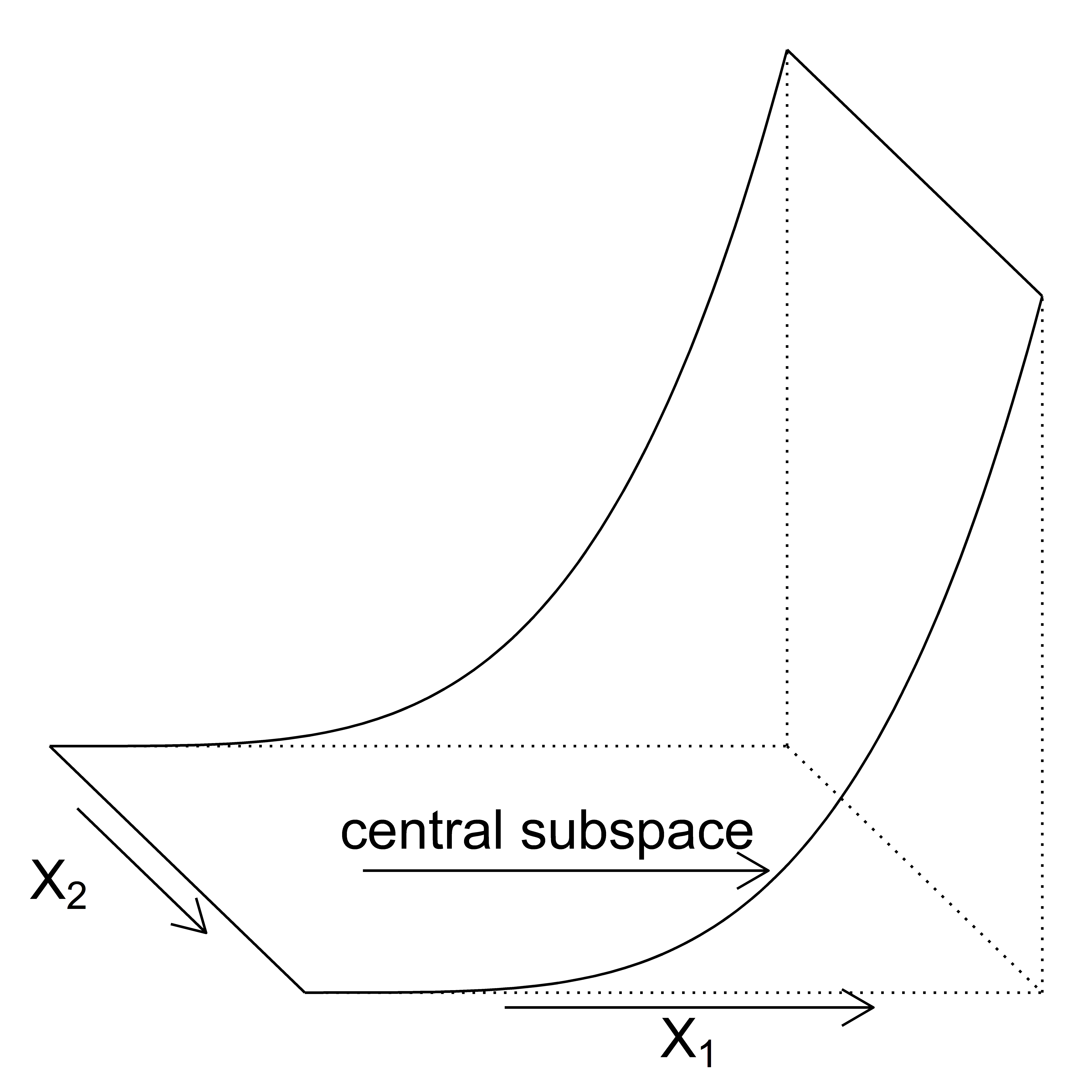
An Illustration

To illustrate the objective of SDR methods, we can look at a simple example. Let $X = (X_1, X_2) \in [0,1]^2$ be a bivariate predictor in the unit square and let $Y \in \R$ be a quadratic function of $X_1$ only. Then, if $\beta = (1,0) \in \R^2$, the outcome $Y$ can be expressed as $Y = \beta^\top X$.

For \[ \begin{split} Y \indep X \mid \beta^\top X \end{split} \]